If two (or more) substances are brought into thermal contact, we observe that spontaneously a certain process, which "automatically" leads to a certain final state, spontaneously occurs. This condition is always characterized by the fact that all the substances involved assume the same temperature. For daily use, it is of interest to understand what determines the final temperature, closer to the temperature of the hottest or coldest substance.

In order to keep the conditions simple, we restrict ourselves to only two substances for the thermal contact in the following experiment. We first place a metal in boiling water at a temperature of about 100 ° C, and in the meantime prepare a thermos flask (calorimeter) in such a way that there is cold water (room temperature) and a temperature probe. There is also a temperature measuring probe in the metal body so that the development of both temperatures can be observed when we immerse the hot metal in the cold water.

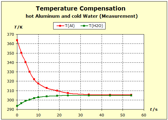
Video: Temperature Compensation Between Hot Aluminum and Cold Water

The hot aluminum has lost very much of its initial temperature, while the cold water has barely warmed. Water is obviously a thermally inert substance, it only slightly changes its temperature.

We repeat the previous experiment but this time take a hot copper block as a metal. We will see whether the nobler metal copper will be able to retain its thermal energy more readily than the aluminum. This would be the case if the final temperature is higher in the following experiment than in the temperature balance between aluminum and water.

Video: Temperature Compensation Between Hot Copper and Cold Water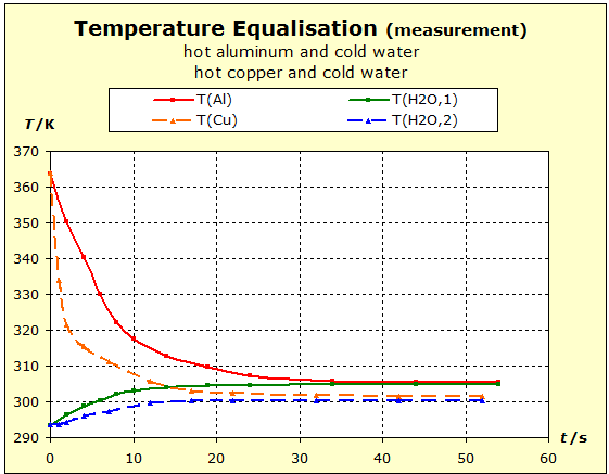

When immersed in the cold water, the two metals at 91°C (364K) have about the same starting temperature and the water is about 20°C (293K) "cold". The two experiments show that water is thermally more inert than metal blocks with the same mass as the water. However, there is also a difference in the thermal inertia between aluminum and copper: in the case of aluminum, the temperature is lowered by about 4 K less than in the case of copper. The aluminum block is thermally more inert than the copper block. The temperature of the water increases with the aluminum more than with the copper: ΔT(water, Al)= 11K; ΔT(water, Cu) = 7K. Therefore, it can be concluded that the aluminum block performs much more (about 57%; 11/7=1,57) thermal work on the water amount than the copper block.

However, it should be borne in mind that, in 100 g of aluminum, about 3.7 mol atoms are present, whereas 100 g of copper is only about 1.6 mol atoms. In our experiments, the thermal inertia of the aluminum is caused by the large atomic number. If one compares the molar standard entropies * of the two substances, the values are found:

S/R(Al)= 3,41

S/R(Cu)= 3,99

The thermal capacities are:

C_p/R(Al)= 2,93

C_p/R(Cu)= 2,94

The thermal capacity of the copper is therefore only very slightly greater than that of the aluminum, so that it is also found from this finding that the thermal inertia of the aluminum in the above experiment is due to the large number of atoms. In sections 3.3 and 3.4, diagrams have already been shown which show systematically for the substances in the periodic system of the elements that the thermal capacities change in the same way, but substantially less, than the molar standard entropies.

* Since the metals do not consist of molecules, the molar entropies have the same numbers as the atomic entropies.

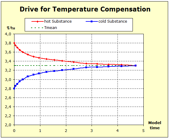
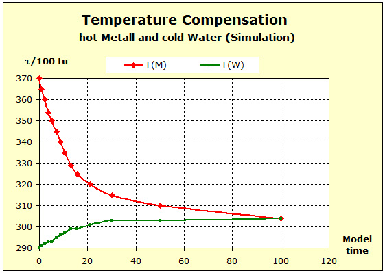
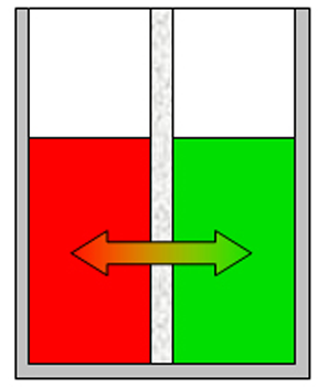
On the model plane the phenomena shown in the previous experiments can be represented in different ways. In the next two videos, the fluid model with beverage bottles is used as a model experiment and the temperature balance between aluminum and water, or copper and water, is reproduced. In both cases, the end temperature is closer to the initial temperature of the substance with the larger standard entropy.
Since the cross-sectional area of the standard entropy corresponds to the fluid model, the bottle with the largest cross-section was used as the model for the water. The bottle with the smallest cross-section corresponds to the copper block.

Video: Model Attempt to Temperature Compensation Between Aluminum and Water

Video: Model Attempt to Temperature Compensation Between Copper and Water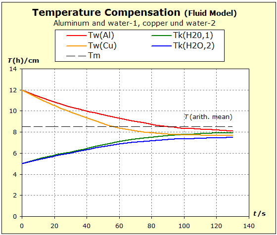

It can be seen from the diagram that the thermal inertia is the greatest in water, and that the aluminum in thermal inertia exceeds the copper because the temperature of the aluminum is not lowered as much as that of the copper The average temperature was plotted. This final temperature is reached only if the standard entropies of both substances are the same.

The fluid model also permits a great simplification, since a spatial representation of the cylindrical storage vessel is dispensed with. Nevertheless, the essential properties of the substances shown, such as entropy / cross-section and temperature / filling height, can be seen. The following link illustrates this.

PDF: Temperature Compensation of two Substances with Different Standard Entropy
(simplified fluid model)

However, if one were to describe the context as comprehensively as possible, one would have to resort to the quantum theoretical bases. This is easy to achieve with the Thermulation-I program. The following animation shows a temperature balance between two different substances such as metal and water, whereby different atomic numbers and the quantum theoretical background of this process can be taken into account. The simulation depicts the process of temperature equilibrium between copper and water, as carried out in the above real-world experiment.

We proceed in six steps:

1. Determination of the standard values of the atomic entropies of aluminum and water

2. Transfer of these real values to the model plane of the Thermulation I program

3. Adjust the real and model values to the two output temperatures of aluminum and water

4. Considering the different atomic numbers of 100g of aluminum and 100g of water

5. Animated visualization of the simulation

6. Assessment of the result

Step 1:
The tables show that, under standard conditions, the molar entropy of aluminum is 28.33 J/(Kmol). Since, in the case of aluminum, 1 mol of the substance consists of 1 mol of atoms, this is already the desired value of the standard atomic entropy S_at(Al). In the case of water it is different. The tables show for the molar standard entropy a value of 69.91 J/(Kmol). Since 1 mole of water consists of 3 mol atoms, this value must be divided by three. Thus, for the water, the atomic standard value of S_at(H₂O) = 23.30 J/(Kmol). The fact that this value for a liquid is smaller than that of the solid metal aluminum requires an explanation. We know, however, that the average atomic mass in the aluminum is 26.98 g/mol, but in the water only 18/3 g/mol = 6 g/mol. The small atomic average mass makes the low entropy of water in comparison with the aluminum comprehensible (the mass rule).

Step 2:
The ration of the two entropy values is:

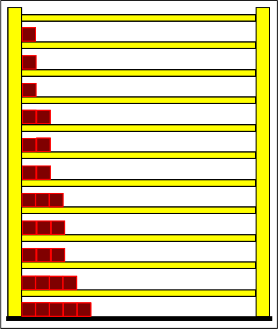
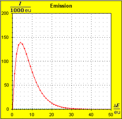
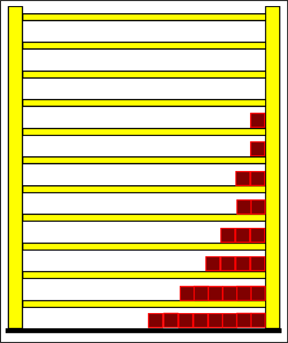
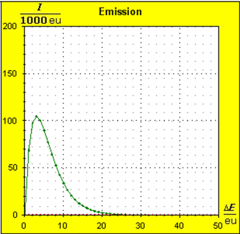
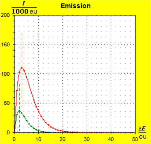
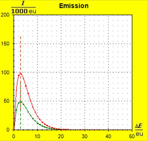
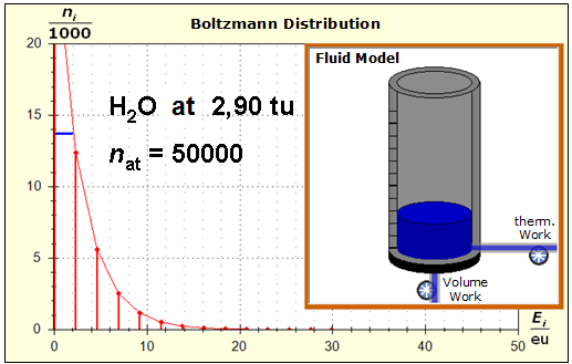
S_at(Al):S_at(H₂O)= 28,33:23,30=1,22:1.

On the model plane, we now have to look for two energy level distances for water and aluminum (equal number of atoms), which lead to such entropy values that adapt well to this ratio. The values ΔE(Al) = 1.7eu and ΔE(H₂O) = 2.3eu fullfill the condition on the model plane in model units well and specifically for about 50000 particles each:

σ(A):σ(B)= 79000 : 64100 = 1,23 : 1

This choice is at first arbitrary, because you could surely find an appropriate entropy ratio on the model plane with two different levels. The goal is to find values that lead to good visualizations in the Boltzmann diagram and the fluid model. Therefore, we now turn to the other constraints that the real substances pretend and then assess in the end whether this choice was neat.

The two following pictures show the standard values of the two modeled substances. The two blue half-value energy lines are visibly equal in length and the temperature scales on the fluid cylinder show the same filling height.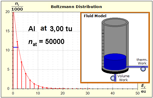

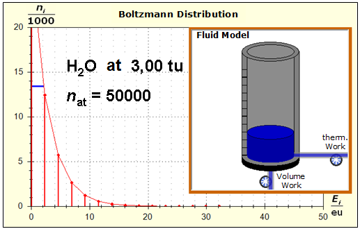It is well to recognize that aluminum has the narrower energy level distances because of the 4.5 times as large atomic mass. Because of the larger cross-section of the fluid reservoir, the greater thermal inertia of the aluminum would be expected.

Step 3: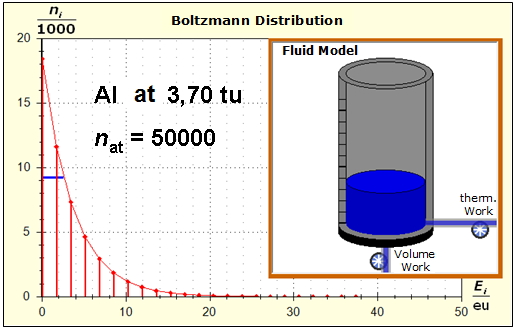
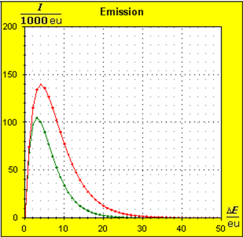
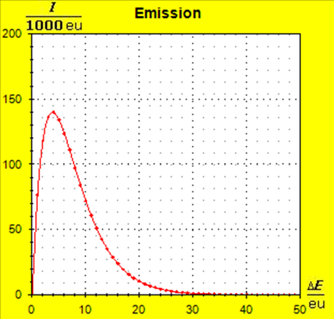
Next we have to bring the two models to their starting temperatures: τ(Al) = 3.70 tu and τ(H₂O) = 2.90 tu. It has already been pointed out above that we can achieve good results on the model plane by dividing the Kelvin temperatures by 100 on transmission to the model. The starting temperature for the aluminum block was the boiling temperature of the water, ie about 370 K and the cold water had a temperature of 290 K (about 20°C.). The model pictures look like this:

Because of the higher temperature in the aluminum (recognizable by the longer blue half-value energy line and the larger filling height), the cross-section, that is, the entropy in the fluid model, has once again increased and thermal inertia increased. In the water, the thermal inertia appears to have diminished somewhat by lowering the temperature.

Step 4:
In this step, we must be clear about the atomic number ratio of the two portions 100g Al and 100g H₂O. To do this we divide the mass 100g by the atomic average masses:

Al :    100g : 26.98 g/mol = 3.71 mol = 3.71 ^. 6e+23 Atome = 2.22e+24

H₂O :    100g : 6.00 g/mol = 16.7 mol = 16.7 ^. 6e+23 Atome = 1.00e+25

These values are transferred in their relation to the model plane by selecting for water the number of 50000 and 11100 atoms for aluminum. Now finally we get the actual starting situation for our model experiment: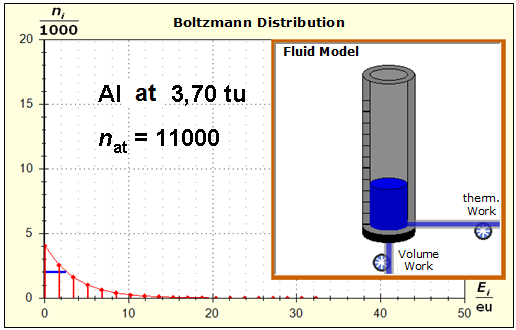

Now, the image has changed significantly: due to the small amount of substance in the case of the aluminum, the entropy and thus the thermal inertia of this metal portion has decreased significantly.

Step 5:
Before we go to the actual simulation, we must bear in mind that we have carried out the experiment in such a way that both substances in an isolated system could exchange thermal energy with one another but not with the environment. In the animated representation the paths are therefore missing, through the mechanical or thermal work in the environment or vice versa.

Animation: Temperature Compensation Between Aluminum and Water

Step 6:
For the temporal representation of the simulation in the following diagram, it was assumed that increasingly longer time spans are required for the transmission of the energy portions during the course of the experiment.

The two diagrams show impressively that the careful determination of the quantum theoretical fundamentals of this simulation led to a suitable representation of the real experiment. For the entropy and its importance for the thermal inertia of a substance, one must consider not only the restoring forces and the particle masses, but additionally the particle numbers as influencing factors.
With the Thermulation-I program, an equally good simulation can also be achieved for the copper water experiment, if the quantum theoretical fundamentals are carefully prepared as in the case of aluminum.

Observing natural processes, which are spontaneous and voluntary, lead to four fundamental questions, which are decisive for the interpretation of the driving phenomenon. How can you understand that

1. the process starts spontaneously?
2. the process speed decreases during the process?
3. the process already may come "at half way to a standstill"?
4. there may also be a drive for a reverse process?

In this section, we will turn to an experiment that is fundamental to understanding the thermodynamic drive. Although the idea of this experiment is very simple, there are still many difficulties in designing the process in such a way that the experimental finding helps us on the way to the thermodynamic drive. The simple idea of the experiment is to say:
We bring two equal amounts of the same substance but with different temperatures into thermal contact with each other and observe the temperature compensation.

At first glance, the result is expected to be that the final temperature is set at the arithmetic mean of the two output temperatures. This is only true, however, if one ignores the fact that depending on the execution of the experiment more or less serious systematic errors are made. Therefore we will discuss the experimental conditions in preliminary considerations.

1. The experiment should be carried out with 50 mL of hot and cold water.
2. We allow the temperature compensation to run in a calorimeter.
3. The calorimeter shall have an intermediate wall. (See picture)

To 1.: It is advisable to choose a liquid substance for the experiment, because determining equally large amount of matter is very easy. Water is easily accessible. However, it must be kept in mind that equal volumes do not contain the same number of atoms at different temperatures. Since the cold water is at room temperature, the density anomaly will not significantly affect the process. Between two solid materials, the thermal contact would be more difficult to produce if, for example, it were metal blocks or larger crystals (candy sugar or the like). Metal powder or powdered crystals would be an alternative.
To 2.: In order to restrict the temperature compensation to the two selected sections of matter and to transferre as little thermal energy as possible to the environment, the experiment is carried out in a calorimeter. However, we must take into account that even the best calorimeter is not a perfectly isolated system and, of course, also calorimeter components are in thermal contact with the two starting materials.
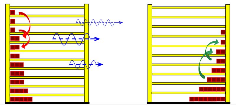
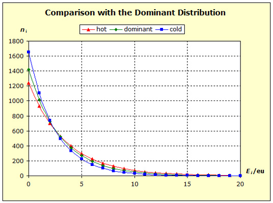
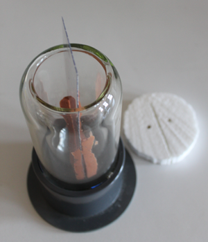To 3. We do not want to mix the two water portions by stiring, and therefore use a calorimeter with an intermediate wall, as is sometimes found in thermo- dynamic textbooks. The quantum theoretical background is as follows: energy is transferred from the higher energy levels of the hotter substance to the lower energy levels of the cold matter. Thus, the number of occupied energy levels, and consequently the entropies, change in both groups of matter.
In order to avoid a discussion about an issue that classical thermodynamics denotes as entropy of mixing, the water portions will not be mixed here. The thermal contact is made via a thin plastic partition. This results in a lower process speed. In the case of two identical substances, even the classical thermodynamics would not expect an entropy of mixing would appear to occur. If we nevertheless exclude the problem of mixing, we can use the same experimental setup for other combinations of substances.
The quantum theory also includes a further aspect: the entropy is composed of different parts and is determined by means of the distribution functions (partition function, state sum) of the translation, rotation, vibration and the electron states. However, a 'partition function of mixture' is not described in the literature.
Another reason to use a shared calorimeter is the interest in the variation of this experiment with two different substances, such as alcohol and water. In those cases, of course, it must be ruled out that the different substances react with one another. Thus, it is known that alcohol and water may react exothermically.

After these preliminary considerations, you can watch the video with the experiment. Since the process speed is low, the experiment takes about 30 minutes. By time-lapse technique the video was staked on about 2 minutes ..

Video with Sound: Temperature Compensation Between Two Water Sections.

The following two diagrams show the measurement data. The temperature curves differ markedly: the upper and lower curves of the water/propan-1-ol pair are higher than the corresponding curve of the water/water pair. In both cases, no definite final temperature is established but thermal energy is radiated during the test period. The highest temperature reached by the cold water is 34.5°C, while the cold alcohol is heated to 38°C. The alcohol is apparently thermally less inert than the water.

In the following two diagrams, a third curve was drawn which shows the arithmetic mean values of the upper and lower temperature curves. The mean temperature drops by almost 0.35 K/min.

Since the cooling of the device has been determined in this way, the cooling effect can be calculated approximately from the measured data. This is shown in the following left diagram.
It is difficult to detect the thermal inertia of the calorimeter because the thermal energy of the water is radiated during the transfer. At the same time this thermal energy of the water heats the calorimeter and as well flows to the environment. However, the arithmetic mean value of the starting temperatures (43.5°C) is certainly an upper limit, up to which the expected end temperature can be assumed for an ideally isolated and noninertial calorimeter.

With this evaluation, we are very close to an expected result in an ideal calorimeter. From this assumption we want to further elaborate the thermodynamic drive to this process.

The left picture shows a Boltzmann distribution for a substance at high-temperature .
As the occupation numbers are only declining slowly, the half-value energy and the temperature are high. The right picture shows a belonging model-emission spectrum. The emission intensity is plotted on the vertical axis as the number of photons emitted per time unit.

We now compare these two representations with the corresponding images for a substance at low-temperature .

The left picture shows a Boltzmann distribution for a substance with the same number of particles as in the previous example but at a low temperature.
Since the occupation numbers decrease rapidly here, the half-value energy is low. A belonging model-emission spectrum is shown in the right picture.

If one compares the spectra of the two examples, one recognizes that the warmer substance provides the higher radiation intensity and that the maximum of its spectrum lies at a higher energy value.

Both substances emit spontaneously according to their temperature. The right picture shows both spectra in one graph. It can be seen that the hotter substance radiates much more thermal energy by emission than the cold substance despite the same number of particles. If both mass portions are present in an outwardly isolated system, both can not prevent the absorption of any radiation in this system. This results in the warmer material also absorbing photons of the colder. If, however, the radiation components are taken into account, the warmer material performs a net thermal work on the colder part. The temperature of the cold increases, the warmer sinks. The emission spectra behave accordingly: the emission of the warmer becomes lower, the emission of the colder becomes stronger. The two radiation maxima approach each other. As long as one substance emits more radiation than the other, there is a drive for spontaneous temperature compensation.
This thermodynamic drive is due to the spontaneous emission.

The above picture summarizes this situation. The warmer substance is described by the left shelf, the colder by the right shelf. The blue sketched photon current represents only the net fraction of the thermal radiation, which is transmitted more from the warmer to the colder. Only this fraction performes thermal work on the colder material.
Since the differences in the intensity of the emissions of the two substances decreases, the thermodynamic drive is also becoming less and less pronounced during the course of the process.
The following animation shows a temporal course of this entire process at the level of the emission spectra.

Animation: Temperature Compensation Between two Substances.

The following diagram also shows the timing of this animation. Compare this graph with the graphs drawn from the measured values, which were shown at the beginning of this section 6.2.

Two further cases of this temperature compensation are still to be discussed:
1. Unequal portions of the same substance
2. Unequal portions of two different substances.

1. In the case of unequal portions of the same substance at different temperatures, it is also expected in an ideally isolated system that the final temperature is no longer exactly the mean temperature. The emission spectra of the initial and final situation show the following two images.

2. For different substances with different temperatures, the difference in the emission curves has to be made clear again. Look at the two following pictures. They show two different substances at the same temperature and number of particles:

The fact that both substances radiate the same number of photons with the same frequencies despite the different level distances is due to the fact that the occupation numbers of the levels are different. At lower distances, occupation numbers are lower, but more levels are occupied. This results in the same number of equal-frequency transitions but out of a larger number of levels.

It should also be pointed out that the entropy rises up to temperature equilibrium. The simulation program yields the entropy increase of the adjacent diagram.
The fact that this is actually a relative maximum can only be simulated with the program, because even after the thermal equilibrium has been reached, further thermal work can still be done on the initially colder, but in the meantime, hotter material. In a real experiment this extra-polated branch of the curve can not be reached.